Throughout this article, I aim to provide with a very simple replicable and practical manual on how to use Genetic Algorithms on optimisation problems. During this, I’ll try to outline the philosophy of applying Genetic Algorithms (GA) and the implications of the many decisions involved in building such algorithms. With this goal in mind, we are going to solve the generalised 8-queens problem using three slightly different customized GA algorithms and comparing its advantages and weaknesses; this way getting a glimpse of the crucial points of building a proper GA model.
By its nature, the N-queens problem is not easily solvable using Genetic Algorithms, and you might finde much more suitable algorithms for this particular problem. Nevertheless, This work might be useful as a general tutorial on learning how to apply GA on any problem.
It is important to note that the purpose of this project is not to achieve the best performance on computational terms neither to construct a model as efficient as possible, but to explore the general considerations involved in the developement of such algorithms and the metrics derived from them. Hence, we’ll use R for its versatility and simplicity when working on ever-changing scripts, providing the more uncomplicated environment for this endeavour.
Genetic Algorithms are a family of algorithms whose purpose is to solve problems more efficiently than usual standard algorithms by using natural science metaphors with parts of the algorithm being strongly inspired by natural evolutionary behaviour; such as the concept of mutation, crossover and natural selection.
When applying genetic algorithms one aims to construct a model that, with some randomness, tries different individuals (possible solutions, differentiated by a list of values that defines its genetic information) to a problem , measure its fitness - which would mean to evaluate whether this possible solutions are perfect solutions or just good to some extent, and to measure this degree of ‘goodness’ - and to make the better solutions to breed and produce a new set of possible solutions with better fitness, and somehow closer to the perfect solution.
This definition is not set in stone and there is some discussion on the classification of different types of algorithms, concerning whether or not they include the crossover part, the mutation or whichever the investigator seems fit to dismiss or include for an specific project. Can be named genetic algorithm an algorithm that has randomly distributed initial population, mutation, natural selection and genetic information being transmited from one generation to the next but it lacks of a crossover? It would be surely included in the label of Evolutionary Algorithms even though it has genes to carry forward. Anyway, we will not enter in such discussions nor delimit our model to the strict definitions of one category or another. This means that we may use terms as genetic algorithm, mutation or crossover as loosely as is reasonable for the sake of the purpose of this project.
This lack of strict mathematical guidance gives the genetic algorithm some freedom to develop heuristic considerations into the build-up of the model. This advantage is also its weakness, for it is a very difficult task to construct a genetic algorithm that converges to the good solutions and not get stuck in solutions that are quite decent but not perfect.
The final solution is then an end product of the best elements of previous generations, carried forward from generation to generation with some degree of randomness (mutation).
Along this work, we will travel through the many decisions that have to be taken in order to construct a proper genetic algorithm and the considerations involved in such decisions, affecting the final performance of the model.
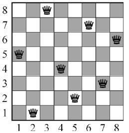
Once we understand what Genetic Algorithm means, we will try to develop a model guided by the principles of this family of algorithms that tries to solve the famous 8-queens problem, and generalised to as many queens as we can. The objective of this problem is to distribute N queens across a NxN chessboard in such way that no queen is able to kill any other queen in the next move.
Knowing this, we have to decide how we do define the position of the queens in a straightforward way. The simplest approach is to use a family of permutations. This is a sequence of 8 unique numbers from 1 to 8 (or N, for the N-queen problem) from which we can construct “brothers” just permutating the position of the elements of the sequence. For instance: (1,2,3,4,5,6,7,8), (5,6,7,8,1,2,3,4) or (8,7,6,5,4,3,2,1). The elements of the sequence has the meaning of the position of each queen. In this way, every element of the array (sequence) represents a row, and from every one of which there is a queen; so the number of every element represents in which column we do put the queen. The solution showed in the image below would be represented as (2,5,7,4,1,8,6,3)
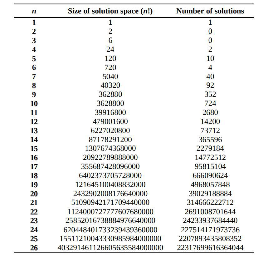
In fact, there are 40320 possible combinations for the 8-queen problems, or N! for N queens. The advantage of using a family of permutations as our individuals is that we do not permit the existence of repeated numbers in the same individual, because that would mean that there are more than one queen in the same row. This considerably minimises the computational effort.
Once we have understood what is an individual and how we do define it, the first question to arise is how do we make them procreate. If we get two different individuals and we pretend to generate a child who is similar to both of them, a general standard procedure is to get some of the elements of the array that defines one of the parents, some other elements of the other parent and mix it together. This is trickier than it may seem, for our individuals are permutations and no repeteated numbers are allowed in its genetic code. There are some algorithms or techniques that allows us to recombinate the genetic information of two parents without repeated numbers, such as the Partially Mapped Crossover.
In this particular problem, the N-queens problem seems obvious that a small change (few permutations) in an individual could lead to an utterly different result for the altered individual. This implies that a son resembling his parents does not have to be similarly good (or bad), for even small changes in the positions of a single queen can lead to a massacre.
For this reason explained, I have decied to present an atypical crossover. This crossover consists in the comparision between the two parents, and to map whose elements of their arrays are equal. We then use this as a mask from which a new individual is created randomly (as the initial population) but remaining untouched those elements that were equal in his parents.
A good example always helps to clarify things: Imagine that we have two parents, P1 = (2,5,1,7,3,4,6,8) and P2 = (2,5,8,6,4,3,7,1). Notice that they have something in commmon, the first element and the second one; then one possible child would be C1 = (2,5,3,6,1,8,7). The child has been generated randomly, but keeping the first position and the second one untouched; this is crucial, because the child carries on unaltered information about his parents. Why is this more useful than a simple recombination? Because we let the algorithm rapidly converge to a solution if those elements the parents had in common were part of a perfect solution, as the stated in the previous example.
There are plenty of other techniques that try different approaches in order to make the algorithm faster or more robust. The ‘Speciation Heuristic’, for instance, penalizes crossover between candidate solutions that are too similar. This encourages population diversity and helps prevent premature convergence to a less optimal solution.
Why is diversity so important? Two parents with a great – but not perfect – fitness can breed excellent – but not perfect – children, whose genetic information that is being carried forward from generations does not and will not pertain to a perfect solution. Thus, lack of diversity would lead the algorithm te get stuck into quite good solutions, but never perfect. Since our crossover has precisely the disadvantage of disencouraging diversity, we’ll try to avoid it using another technique. We’ll add mutation.
Clarification: At this point would be relevant to point out that we are making use of loose terminology. So, in order to not piss some people off, I’d like to clarify the usage of some terms. First, the definition of the crossover is actually quite controversial and it triggers some utter discussions. The usage we are doing of the term might not be fitting the formal definition of a crossover, you should think about it as some kind of heuristic function that involves the resemblance of both parents and some degree of randomness, but not exactly a crossover, because it does not interchange genetic material. Consequently, a genetic algorithm without a proper crossover maybe should actually not be called genetic at all, and use another more generic label as Evolutionary Algorithm. We’ll keep talking about crossover and genetic algorithm from this point onwards anyway.
So we don’t want to get stuck in local minima. In order to avoid that, some degree of randomness is needed to escape from those pretty decent individuals. And for this purpose it is useful the concept of random mutations. A typical and very simple mutation consists in permutate two elements of the genoma of an individual. When and where to apply the mutation is chosen randomly and is one of the crucial parameters to balance between a more exploratory or a more elitist model.
For our situation, we have chosen a weird crossover method with a great risk of falling into local minima; and for this reason we have chosen an also a weird mutation. The mutation that we will apply in our models is considerably more aggressive than the usual, for just one permutation may not let us escape from a whole family of inbreeded quite decent individuals with many elements in common but bearing no hope for a future perfect grandson.
The mutation used in our models is, then, a complete rearrangement of the genoma of an individual when it is created. That means that every time a couple procreates and produces a child, this individual has a chance to be generated randomly, with no regard for parents resemblance whatsoever.
Another possible solution for this would have been the standard usual mutation but with higher probabilities of occurring. This could make sense and it is a very reasonable solution; but considering the approach taken before, in which we stated that smaller changes can lead to utterly great differences in fitness, making minor changes very often would be more chaotic in our population developement than a rather improbable major change.
Using the same example with parents P1 and P2 (the same as before), a child of this parents that suffers a mutation could be Cm = (8,1,6,2,7,5,3,4).
Now that we know how the individuals can procreate and breed, we need to decide which of them will do it. We have to set a rule to establish a hierarchy between individuals, so only some of them are able to produce offspring.
The number of solutions for the 8-queens version is $92$. This number increases greatly for larger $N$s, and there is no closed formula to predict the number of unique solutions for any given $N$, even though there is a known sequence for it. Considering that we aim to generalise this problem for many more queens than $8$, simply counting the number of dead queens would be misleading when comparing the success of the solutions and could complicate the interpretations derived from the metrics of the model.
The most common and reasonable way to address this is to define a fitness function. The fitness is telling us, in some sense, how good this individual is. Provided that our goal is to obtain an individual with 0 dead queens, we could set our fitness function as the inverse of the number of dead queens. Or
if we want to avoid divergences. This way, our fitness function reaches a maximum of F=1 whenever the number of dead queens is 0.
Now we know how to establish a hierarchy between the individuals. The first move we make is to create a random initial population of the family of permutations of size $N$. How big is this initial population is a point of great interest but in which we will not focus. Too small population would lead to a less diverse population, and a too large population would lead to an overload of the memory and a lot of redundant time consumption for each computation. So in order to keep this analylsis simple we define a formula to set the initial population as $P = 2Q^2$, where $P$ is the size of the population, and $Q$ is the number of queens of the problem. This way, we maintain a population size in accordance with the magnitude of the problem. Once we have the initial population, the point of the following process will be to select, based on the fitness function, which indiviuals of this population will have the chance of procreating and perpetuate its genetic information.
There are many different approaches to select the creators of the new generation. Some set a probability to procreate based on the fitness; others kill a bunch of low fitted individuals before they can reproduce. Some models let the individuals generate offspring again and again along the newer generations, if they survive the purge; whereas others models just let the parents to breed once and then they die. One thing is certain, and that the number of toddlers by couple and the extremism of the purge when killing individuals are parameters that have to be considered together, because a disbalance of this two mechanisms can lead to a premature extinction of the population - finalising the program; or worst, to an ever-growing population that can overload the RAM memory of our computer.
For this project we tested three very different models of purging the population, all of them under the same heuristics that we are calling crossovers that we have already discussed. Now we will talk a bit about these different methodologies, its implications, its limitations and its advantages and how they play with our crossover.
This method essentially consists on killing all population except the two fittest individuals. These two survivors will produce a new entire population based on its genetic information. The point here is that this couple has so many toddlers that the new population is as numerous as the previous one.
The point of this kind of method for deciding who are the survivors of the purge is an interesting synergy with the philosophy of our crossover. If Adam & Eve survived the purge it is because they were the best individuals, if they had something in common it maybe is because it forms part of a perfect solution; this way the model converges extremely fast to a good solution. But, as we have discussed, good is not perfect. The disadvantage of this kind of this kind of models is that they are highly exploitative and so they get stuck very rapidly on a good solution, yet is improbable that they find a perfect one.
We can tune the model into a one more exploratory with lower risk of getting stuck on a non-perfect solution if we increase the chance of mutation. As we have discussed, our mutation process is highly exploratory; so if we rise the probability of this a bit, we might find some delicated equilibrium between this combination of both extremely exploratory and extremely exploitatory measures.
# Declaring functions needed to compute Genetic Algorithms --------------------------

# Find common pattern in parents (function)
noncommon <- function(par1,par2){
	noncommon <- which(!par1-par2 == 0)
}

# Generate offspring (function)
gen.offspring <- function(par1,par2, noff, pmut){
	for (j in 1:noff){
		offseed <- sample(par1[noncommon(par1,par2)])
		randomdummy <- runif(1)
		if (randomdummy<=(1-pmut)){
			for (i in 1:nproblem){

				if (i %in% noncommon(par1,par2)) {
					son[i] <- offseed[1]
					offseed <- offseed[-1]
				}
				else {son[i] <- par1[i]}
			}
		}
		else {son <- sample(par1)}
		offspring[[j]] <- son
	}
	return (offspring)
}

# Measuring fitness (function)
meas.error <- function(subject){
	error <- 0
	for (i in 1: length(subject)){
		x <- i
		y <- subject[i]
		for(j in 1:length(subject)){
			if (i !=j){
				dx <- j
				dy <- subject[j]
				if (abs(dx-x)==abs(dy-y)){error = error+1}
			}

		}
	}
	return(error)
}

kill <- function(population,pmut,mort){
	newpopulation <- list()
	b <- length(population)
	a <- 1
	while(a < b & length(population)>1){
		w1 <- sample(population,1)[[1]]
		w2 <- sample(population,1)[[1]]

		newpopulation[[a]] <- fight(w1,w2,pmut,mort)
		a <- a+1
	}
	return(newpopulation)
}


# Declaring parameters and executing model --------------------------


# Magnitude of the Problem (Number of queens)
nproblem <- 10

# Probability of mutation
pmut <- 0.3

# Seed for generating initial parents
seed <- seq(nproblem)

# List to be filled
offspring <- list()

# Arrays to be filled
son <- c()
subject <- c()
fitness <- c()
max.fitness <- c()

# Number of toddlers by couple
noff <- nproblem*5

# Initial parents
par1 <- sample(seed)
par2 <- sample(seed)


b <- 0
# Creating further population ---------------------------------------------------
repeat{
	# Measuring fitness of every child
	for (i in 1:noff){
		offspring[[i]] <- gen.offspring(par1,par2,noff, pmut)[[i]]
		subject <- offspring[[i]]
		fitness[i] <- (1/(1+meas.error(subject)))
	}

	# Selecting most fittest childs as new parents
	par1 <- offspring[sort(-fitness,index.return=TRUE)[[2]][1]][[1]]
	par2 <- offspring[sort(-fitness,index.return=TRUE)[[2]][2]][[1]]
	max.fitness <- append(max.fitness, max(fitness))

	b <- b+1

	if (max(fitness)== nproblem*(nproblem-1)) break
	if (b > 5000) break
	if (max(fitness) == 1) break
}
I didn’t get with a fancy name this time.
Another way to address this problem is to tweak a bit our first method and be more magnanimous with the population, letting survive not only two individuals, but half of the entire population. Which half? The lest fitted half. Killing the worst half of the population let us continue with the philosophy of combining individuals which are the best, and use on them a crossover that remarks those characteristics that made them the best individuals in town. This way, improving the general fit of the next population. In this case though, letting far more individuals to breed, we are openning the solutions space to different families of individuals, increasing the variability between individuals. This saves us of converging into local minima - that is, getting stuck with quite decent but non-perfect individuals.
Once we have several individuals ready to procreate, another important decision is to set how we make couples out of them. There are many different approaches to address this point. Some models pair the individuals randomly but with exclusivity - that is, any couple can just procreate between them and one time. Some others make couples out of individuals with similar fitness, so this way it guarantees some degree of inbreeding. Different models do exactly the contrary, they pair the survivors priorizing those couples with great differences between their fitness value, facilitating diversity within the population.
In our case, we will make it more simple. We have just selected random couples with exclusivity. This way we can easily tune the number of toddlers by couple in order to predict the size of the future populations. Moreover, it makes sense that we aim to avoid strategies derived from considerations such as “similar fitness implies similar individuals”.
In the future, we may call this model just Half, for simplicity.
# Declaring functions needed to compute Genetic Algorithms --------------------------

# Find common pattern in parents (function)
noncommon <- function(par1,par2){
	noncommon <- which(!par1-par2 == 0)
}

# Generate offspring (function)
gen.offspring <- function(par1,par2, noff, pmut){
	for (j in 1:noff){
		offseed <- sample(par1[noncommon(par1,par2)])
		randomdummy <- runif(1)
		if (randomdummy<=(1-pmut)){
			for (i in 1:nproblem){

				if (i %in% noncommon(par1,par2)) {
					son[i] <- offseed[1]
					offseed <- offseed[-1]
				}
				else {son[i] <- par1[i]}
			}
		}
		else {son <- sample(par1)}
		offspring[[j]] <- son
	}
	return (offspring)
}

# Measuring fitness (function)
meas.error <- function(subject){
	error <- 0
	for (i in 1: length(subject)){
		x <- i
		y <- subject[i]
		for(j in 1:length(subject)){
			if (i !=j){
				dx <- j
				dy <- subject[j]
				if (abs(dx-x)==abs(dy-y)){error = error+1}
			}

		}
	}
	return(error)
}

kill <- function(population,pmut,mort){
	newpopulation <- list()
	b <- length(population)
	a <- 1
	while(a < b & length(population)>1){
		w1 <- sample(population,1)[[1]]
		w2 <- sample(population,1)[[1]]

		newpopulation[[a]] <- fight(w1,w2,pmut,mort)
		a <- a+1
	}
	return(newpopulation)
}


# Declaring parameters and executing model --------------------------

# Number of toddlers by couple
noff <- 4

# Magnitude of the Problem
nproblem <- 13

# Probability of mutation
pmut <- 0.1

# Mortality
mort <- 0.45

# List to be filled
offspring <- list()
population <- list()

# Arrays to be filled
son <- c()
subject <- c()
fitness <- c()
av.fitness <- c()
max.fitness <- c()

# Count Variables
b <- 0
ind <- 0

# Initial Population ------------------------------------------------------
ipop <- (nproblem)^2*2
for(i in 1:ipop){
	population[[i]] <- sample(seq(1:nproblem))
}

# Reproduction ---------------------------------------------------

repeat{
	m <- 1
	ind <- ind + length(population)
	while(length(population)>1){
		# Selecting parents from population
		par1 <- population[[1]]; population <- population[-1]
		par2 <- population[[1]]; population <- population[-1]

		# Measuring fitness of every child
		for (i in 1:noff){
			offspring[[m]] <- gen.offspring(par1,par2,noff,pmut)[[i]]
			subject <- offspring[[m]]
			fitness[m] <- (1/(1+meas.error(subject)))
			m <- m+1
		}
	}

	# Performance measures
	av.fitness <- append(av.fitness, mean(fitness))
	max.fitness <- append(max.fitness, max(fitness))

	# Get the most fittest individual
	bestguy <- offspring[max(fitness,index.return=TRUE)]
	if (max(fitness) == 1) {
		print <- 'SUCCESS!'
		break
	}

	# Kill all parents
	population <- list()
	rm(par1,par2)

	# Populating the new world
	a <- round(length(offspring)*(1-mort)*0.5)*2
	k <- 1
	while (length(offspring) != 0){
		population[[k]] <- offspring[[max(fitness,index.return=TRUE)]]
		fitness <- fitness[-max(fitness,index.return=TRUE)]
		offspring <- offspring[-max(fitness,index.return=TRUE)]
		k <- k +1
		if(k > a) break
	}
	b <- b+1
	offspring <- list() # Kill all children not fitted enough

	if (b > 5000) {
		print <- "FAILURE"
		break
		}
	if (length(population)<2){
		print <- 'EXTINCTION'
		break
	}
}
This last method is a bit funny. The Great Tournament is a strange version of a standard methodology that we have not yet discussed, that is the tournament selection.
A tournament essentially consists in selecting randomly a bunch of individuals and make them fight; and the result of this battle will decide which of them survives the purge. The most obvious way to decide the winner is to compare its fitness value; the victorious figther would be he who was the greater fitness. Another approach, more exploratory, would be simply to set a probability of victory biased towards the more fittest individual.
As a clarification; imagine selecting 10 random individuals out of the entire population and making them to fight, one of them comes out as the mighty winner and goes into a dating pool to mate; then select another set of 10 random individuals and make them fight, select a winner, put him into the dating pool, and iterate. Once we have a dating pool plenty of proud champions, we make them breed and generate an entire new generation.
Some simple tweaks that can be performed on the tournament method are changing the battle size; we can make 3, 10 or 100 individuals fight each other. There may be more than one winner, too. And what about the losers? Can they have the chance to get involved in another fight again and try to win this time, or we just kill them?
These changes have a great impact on the performance of the final algorithm; for example, a larger tournament size implies a higher selection pressure, which turns in a more elitist model.
For our study, we have selected battle size of just $2$ oponents. In this fight, the individual of higher fitness has a chance of winning of an $85\%$, whereas the weaker individual has a $15\%$ (obviously), with no regard on how big or small is the difference between their fitness.
To this simple method, I have decided to add an interesting tweak that we’ll give some kind of a second chance with the loser. If the stronger individual wins the battle, he is the survivor and he is sent to the dating pool to populate the new generation. But if the weaker individual is the one who wins, he does not survive the purge; he just mates with his opponent and gets a child, and this child is the one sent to the dating pool in order to populate the new generation, with his father/mother.
This weird method has both exploratory characteristics - because of its small tournament size - and exploitatory ones - because of the impossibility for the weaker individual to carry forward its genetic information without mating his rival.
The point again is to create some balance between exploratory and exploitatory characteristics that leads to a reasonable equilibrated model.
# Declaring functions needed to compute Genetic Algorithms --------------------------

# Find common pattern in parents (function)
noncommon <- function(par1,par2){
	noncommon <- which(!par1-par2 == 0)
}

# Generate offspring (function)
gen.offspring <- function(par1,par2, noff, pmut){
	for (j in 1:noff){
		offseed <- sample(par1[noncommon(par1,par2)])
		randomdummy <- runif(1)
		if (randomdummy<=(1-pmut)){
			for (i in 1:nproblem){

				if (i %in% noncommon(par1,par2)) {
					son[i] <- offseed[1]
					offseed <- offseed[-1]
				}
				else {son[i] <- par1[i]}
			}
		}
		else {son <- sample(par1)}
		offspring[[j]] <- son
	}
	return (offspring)
}

# Measuring fitness (function)
meas.error <- function(subject){
	error <- 0
	for (i in 1: length(subject)){
		x <- i
		y <- subject[i]
		for(j in 1:length(subject)){
			if (i !=j){
				dx <- j
				dy <- subject[j]
				if (abs(dx-x)==abs(dy-y)){error = error+1}
			}

		}
	}
	return(error)
}

kill <- function(population,pmut,mort){
	newpopulation <- list()
	b <- length(population)
	a <- 1
	while(a < b & length(population)>1){
		w1 <- sample(population,1)[[1]]
		w2 <- sample(population,1)[[1]]

		newpopulation[[a]] <- fight(w1,w2,pmut,mort)
		a <- a+1
	}
	return(newpopulation)
}


fight <- function(w1, w2,pmut,mort){
	e1 <- meas.error(w1)
	e2 <- meas.error(w2)

	if(e1 > e2) {
		a <- runif(1)
		if(a < mort) vic <- w2
		else  vic <- gen.offspring (w1,w2,1,pmut)[[1]]
	}
	if(e1< e2){
		a <- runif(1)
		if(a< mort) vic <- w1
		else vic <- gen.offspring (w1,w2,1,pmut)[[1]]
	}
	if(e1 == e2) vic <- gen.offspring (w1,w2,1,pmut)[[1]]
	return(vic)
}

# Declaring parameters and executing model --------------------------

# Number of toddlers by couple
noff <- 5

# Magnitude of the Problem
nproblem <- 10

# Probability of mutation
pmut <- 0.01

# Mortality
mort <- 0.5

# List to be filled
offspring <- list()
population <- list()

# Arrays to be filled
son <- c()
subject <- c()
fitness <- c()
av.fitness <- c()
max.fitness <- c()

# Count Variables
b <- 0
ind <- 0

# Initial Population ------------------------------------------------------
ipop <- (nproblem)^2*2
for(i in 1:ipop){
	population[[i]] <- sample(seq(1:nproblem))
}

# Reproduction ---------------------------------------------------

repeat{
	m <- 1
	ind <- ind + length(population)

	# Measuring fitness of every member of the population for statistical purposes
	for (i in 1:length(population)){
		subject <- population[[i]]
		fitness[i] <- (1/(1+meas.error(subject)))
	}


	# Performance measures
	av.fitness <- append(av.fitness, mean(fitness))
	max.fitness <- append(max.fitness, max(fitness))

	# Get the most fittest individual
	bestguy <- population[max(fitness,index.return=TRUE)]
	if (max(fitness) == 1) {
		print <- 'SUCCESS!'
		break
	}

	# Killing festivity
	population <- kill(population,pmut,mort)
	b <- b+1

	while(length(population)>1){
		# Selecting parents from population
		par1 <- population[[1]]; population <- population[-1]
		par2 <- population[[1]]; population <- population[-1]
		for(i in 1:noff){
			offspring[[m]] <- gen.offspring(par1,par2,noff,pmut)[[i]]
		}
		m <- m+1
	}

	population <- offspring

	if (b > 5000) {
		print <- "FAILURE"
		break
	}
	if (length(population)<2){
		print <- 'EXTINCTION'
		break
	}
}
Now that we have constructed completely our Genetic Algorithms, it is important to be aware of how well they perform. In computational problems, it is usual to mean fast when we say good; so the point of this chapter is to evaluate the speed in which our algorithms manage to find a perfect solution.
As stated in the abstract, we are using an inefficient programming language. So the computing time required for any process would be much larger than with many others languages such as “C” or “Fortran”. Hence, the point of the measurment of performance of our algorithms has to be something that can be extrapolated to many others programming languges, or to a more efficient programmer; hoping that some of these algorithms will be transcribed in such way that they may be more useful for direct application.
For this reason, the performance metric that we will be measuring all the time will be individuals. Along all the algorithms we are generating tons of individuals, and every individual is a trial to get the very solution of the problem. Thus, the fewer individuals a program has to generate in order to get the proper solution the more efficient it is. How much time it takes to generate every individual is a problem essentially regarding the programming language and the diligence in which the program is coded; effort that lands outside the scope of this project.
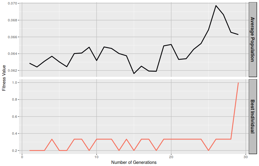
Another perspective to analyse the performance of a Genetic Algorithm is to measure the time evolution of the average fitness of its population from generation to generation, or the time evolution of the fitness of the best invidiual of each generation. Ideally, a proper algorithm tens to consistently improve those metrics over generations.
Now that we know what to measure, we must measure it. In order to do that, we run those models over different number of queens, with different numbers of probability of mutation and as many times as it has been plausible. Then all data is recorded and stored for its analysis. This can be done with the bunchs of code stated above. It might take a few hours to compute everything, so I’d recommend to let it running overnight.
Once we have all the data generated, we just need to loaded and clean it a little bit for proper visualisation.
We’ll start theh analysis looking at the data without making distinction between the models.
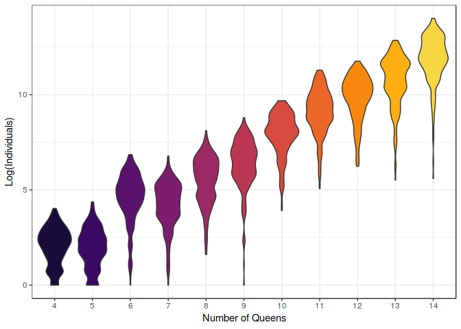
df %>%
	filter(model != "random") %>%
	ggplot(aes(x=as.factor(nqueens), y = log(ind), fill = as.factor(nqueens))) +
	geom_violin(bw=0.2, scale="area") +
	scale_fill_viridis(discrete=TRUE) +
	labs(x = "Number of Queens", y = "Log(Individuals)") +
	theme_bw() +
	theme(legend.position="none")

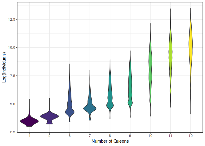
If we look at the figure above, we can appreciate the increase in computational effort when we rise the number of queens of the problem to solve. One interesting thing about these kind of plots is that we can appreciate the distribution of the results, and notice that not only increases the computation needed to solve a problem, but the dispersion of the results. This means that it is harder to predict the time needed to get a solution.
If we want to dig a little deeper, we can split these results from the different models used each time we run the program.
df %>%
	filter(model != "random") %>%
	ggplot(aes(x=as.factor(nqueens), y = log(ind), colour = as.factor(model))) +
	geom_jitter() +
	scale_colour_viridis(discrete=TRUE) +
	labs(x = "Number of Queens", y = "Log(Individuals)", colour = "Model") +
	theme_bw()

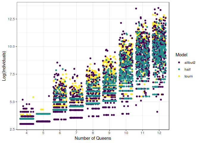
In this figure, we can notice how different they behave. It can be seen that the tourn (which is the Great Tournament model) behave much more chaotically than the other two. Moreover, it seems that usually the half model and the allbut2 (Recursive Adam \& Eve) tend to be quicker finding the optimal solution. This happens for a number of queens lower than $10$, once we have reached that level of difficulty, the results start to be messy and somehow less predictable.
So far, we have seen the relation between the Number of Queens of the problem and the computaional effort. It would be interesting to analyse now the effect on performance of the probability of mutation. We constructed this possibility, when building the model, in order to compensate some of the most elitistic characteristics of our models. It could be interesting how the value of this parameters affects the results.
df %>%
	filter(model != "random") %>%
	ggplot(aes(x=as.factor(nqueens),y=as.factor(mutate))) +
	geom_tile(aes(fill=log(ind))) +
	facet_wrap(~model) +
	scale_fill_viridis(discrete=FALSE) +
	labs(x = "Number of Queens", y = "Mutation Probability", fill = "Log(Individuals)") +
	theme_bw()

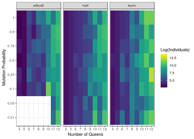
If we now take a look at the figure above, we can notice the major differences between the models, and how differently they make use of the probability of mutation. The biggest influence can be seen in the allbut2 model. In fact, smaller probabilities of mutation such as $0.01$ or $0.05$ have been to be removed from the analysis because this model took so much time to compute even the smaller problems that the collection of relevant data was not feasible. This issue remarks the great importance of mutation in the construction of so very exploitatory models. Actually, it might be noticed that it behaves better when this probability is increased; achieving some kind of sweetspot around $p=0.5$.
Nevertheless, it is also relevant to point out how unconnected the probability of mutation and the performance of the half model and the tournament model they seem. The number of individuals needed to find a solution does not seem to depend on the probability of mutation whatsoever.This kind of insight is extremely useful developing this kind of algorithms.
Despite all this fancy algorithms, we also know that is always possible to solve the N-Queens problem using the simplest and savagest method available, just trying combinations at random until one of them happens to be perfect and outputs $F = 1$. How probable is that? It depends on the dimensions of each problem. If we look back at the table of the solucions space we can see the number of possible unique individuals, with the number of unique perfect solutions of the problem. This way we can find out the an expected number of individuals needed to get a perfect solution.
More practically, we could just plainly generate random permutations of the individuals until one of them happens to be the perfect solution. Then record how many trials have been necessaries, and iterate until we have enough data to compare the results.
df %>% # Used
	filter(model == "random") %>%
	ggplot(aes(x=as.factor(nqueens), y = log(ind), fill = as.factor(nqueens))) +
	geom_violin(bw=0.25) +
	scale_fill_viridis(discrete=TRUE, option = "B", begin=0.1,end =0.9) +
	labs(x = "Number of Queens", y = "Log(Individuals)") +
	theme_bw() +
	theme(legend.position = "none")

Note that this plot is in logarithmic scale. See how rapidly the computational requirements increase over the difficulty of the problem.
Now the interesting point is to compare the performance of our models with the random selection, as shown in the figure below. In this graph can be seen how much better the random selection performs, compared to our models. This is kind of disencouraging at first sight, but note that as we increase the difficulty of the problem, our models start to be relatively more useful and eventually surpasing the power of randomness.
df %>%
	filter(nqueens != 13 & nqueens != 14 & nqueens > 3) %>%
	filter(mutate !=0.01 & mutate !=0.05) %>%
	ggplot(aes(x=as.factor(nqueens), y = log(ind), fill = as.factor(model))) +
	geom_violin(bw = 1) +
	scale_fill_viridis(discrete=TRUE) +
	labs(x = "Number of Queens", y = "Log(Individuals)", fill = "Model") +
	theme_bw()

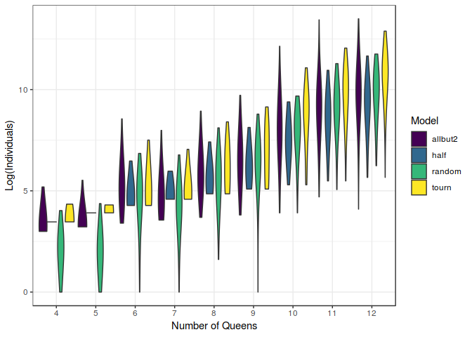
These results might reinforce the idea that complex optimisation schemes such as Genetic Algorithms might be useful just for extremely complex problems. In our case, for a number of queens greater than $10$.
At first sight, the utility of this measurement might not appear so obvious, but it may be remarkable to know whether a population of solutions tends to improve consistently from generation to generation or it justs bounds randomly until some lucky guy hits the jackpot and it just happens to be the perfect solution. Ideally, a proper model should provide a steady ascending curve describing the average fitness of the population across generations.
Along this article, we have seen the implications of each decision made when constructing a genetic algorithm model. We have noticed how unalike the performance can be when using differnet survival models and how differently they interact with mutation.
For lower number of queens, we have noticed the superiority of the Kill Half of the Population and Recursive Adam \& Eve models over the the Great Tournament; despite that random selection outperformed all of them. From number of queens higher than $10$ the results have shown a more unpredictable behaviour, and is not quite clear whether or not made-up models as ours are more useful than simple random trial and error, but the results are quite encouraging, and with theh gradual increase in overall fitness in the population, is not unreasonable to sugggest that the model would perform much better than randomness for even higher number of queens.
The parameters involved – such as mutation probability – have been of great importance for the most elitistic model (the Recursive Adam \& Eve) but of little importance for the other two.
This thought opens up another point of the results that ought to be considered. The main parameter studied in this project has been the mutation probability, and they have not shown quite clearly whether this parameter has a relevant effect on the performance of the models. The common characteristic of each of the models was their “crossover”. Moreover, the mutation probability, in the way that has been created, can be thought as the probability that the crossover does not actually occur when producing a new child; and it is just created randomly. This leads to the conclusion that it is not plainly clear whether our “crossover” method does have a relevant effect in the developement of future generations or not. The only exception for that has been showed when using very little mutation probability on the allbut2 model; in that case the program got stuck in local minima partly as a cause of this “crossover”. Nevertheless, occasional solutions have been found using the allbut2 with a moderate mutation probability ($0.25 < p < 0.75$) that largely outperformed the rest of the models. In some sense, we can think that this model, using this “crossover” is so elitistic that converges rapidly to a solution, regardless of whether it is perfect or not; so it is not strange that sometimes finds a perfect solution faster than the rest.
We do not have clear enough results to conclude whether or not these Genetic Algorithm models are more useful finding N-Queens solutions than a random trial and error, for higher number of queens. And it is clear than the trial and error performs far better than our models, when applied on lower number of queens.
Despite this discouragment, further investigation can be made applying these models on even higher number of queens, in different problems or using different “crossovers”. Future research should also dig deeper on the importance of different parameters such as the population size, for this variable makes a great difference in the performance of this and other models.
If you have enjoyed this article, you might be interested in reading further on Genetic Algorithms. Genetic Algorithms is a kind of optimisation algorithm that is englobed within the concept of metaheuristics. For anyone interested in the subject, I highly recomment the following books. I can not stress enough how useful they are.
Written on 06 Sep 2018 by Alejandro Jiménez Rico