One of the most common financial advices that you can hear in every christmas meal is that you should be saving a fixed amount of money each month. Not only that, but you should avoid pre-cooked schemes offered by your bank and simply invest your savings in the stock market. Investing in the U.S. market or even the global stock market has been a wise decision if you look at the long term (more than 10 years), even if you invested in peak of any pre-crisis crest.
So it seems that saving some money and investing it in stocks looks like a good idea. Great. Now, which market should you invest in? Which stocks? A safer approach to that is just buying an ETF and follow the trend of some index. At the end you are putting your money in the general behaviour of the market. If the economy does well, you’ll do well. Otherwise, you could try to figure out which firms will exceed the market. In this article I will outline a way to test different strategies to base that decision on, using quantitative analysis of the financial statements.
Even though both claim to be quantitative, I need to stress the difference between what I will suggest and the famous Technical Analysis (TA). TA is built on historical price developments and believes that certain patterns on price history may be identified and used to predict future movements of the quotes. TA focuses on how investors’ behaviour might push prices in the future based on historical patterns.
In contrast with that, Fundamental Analysis (FA) focuses on the firm and the value of the ownership right itself, rather than on the market price of it. It established a defined difference between Value and Price. And it believes that the Price tends to reflect Value in the long term. Hence, it claims that the fair value can be computed from the future cash flows, debt, strategic position or future plans.
There is a huge and broad field on fundamental analysis that covers a lot of different perspectives of a firm; some of them quantitative and some others qualitative. One of the quantitative is the study of the financial statements of the firms.
Now, we’ll get down to business.
In order to begin, we need data. We want to try out how we can compute the financial statements of firms to decide in which we should invest our savings. Therefore, we need those financial statements.
From now on, we will be making use of some R packages:
library(tidyverse)
library(data.table)
library(quantmod)
library(rvest)
library(progress)
library(lubridate)
library(feather)
library(zoo)
Firstly, we need a list of the stock universe that we will be considering. For simplicity, I constructed this making use of the widest indexes of the Standard \& Poors.
getTickers <- function(){
	sp500_wiki <- read_html(
		"https://en.wikipedia.org/wiki/List_of_S%26P_500_companies")

	symbols_table <- sp500_wiki %>%
		html_nodes(xpath='//*[@id="mw-content-text"]/div/table[1]') %>%
		html_table()

	symbols_table <- symbols_table[[1]]
	tickers <- as.character(symbols_table$`Ticker symbol`)

	sp1000_wiki <- read_html(
		"https://en.wikipedia.org/wiki/List_of_S%26P_1000_companies")

	symbols_table <- sp1000_wiki %>%
		html_nodes(xpath='//*[@id="mw-content-text"]/div/table[3]') %>%
		html_table()

	symbols_table <- symbols_table[[1]]
	tickers2 <- as.character(symbols_table$`Ticker Symbol`)

	tickers <- c(tickers,tickers2)

	for(i in 1:length(tickers)) tickers[[i]] <- gsub('\\.', '-', tickers[[i]])

	return(tickers)
}
With this function getTickers() we’ve got a complete list of the tickers of 1500 companies, including 500 from the SP500. Now, we’ll use these stickers to get the financial statements from each one of the companies.
getFinancials <- function(ticker){
	stock <- ticker
	output <- tibble()

	for (i in 1:length(stock)) {
		tryCatch(
			{
				url <- "https://finance.yahoo.com/quote/"
				url <- paste0(url,stock[i],"/financials?p=",stock[i])
				wahis.session <- html_session(url)
				p <-    wahis.session %>%
					html_nodes(xpath = '//*[@id="Col1-1-Financials-Proxy"]/section/div[3]/table')%>%
					html_table(fill = TRUE)
				IS <- p[[1]]
				colnames(IS) <- paste(IS[1,])
				IS <- IS[-c(1,5,12,20,25),]
				names_row <- paste(IS[,1])
				IS <- IS[,-1]
				IS <- apply(IS,2,function(x){gsub(",","",x)})
				IS <- as.data.frame(apply(IS,2,as.numeric))
				rownames(IS) <- paste(names_row)
				temp1 <- IS
				url <- "https://finance.yahoo.com/quote/"
				url <- paste0(url,stock[i],"/balance-sheet?p=",stock[i])
				wahis.session <- html_session(url)
				p <-    wahis.session %>%
					html_nodes(xpath = '//*[@id="Col1-1-Financials-Proxy"]/section/div[3]/table')%>%
					html_table(fill = TRUE)
				BS <- p[[1]]
				colnames(BS) <- BS[1,]
				BS <- BS[-c(1,2,17,28),]
				names_row <- BS[,1]
				BS <- BS[,-1]
				BS <- apply(BS,2,function(x){gsub(",","",x)})
				BS <- as.data.frame(apply(BS,2,as.numeric))
				rownames(BS) <- paste(names_row)
				temp2 <- BS
				url <- "https://finance.yahoo.com/quote/"
				url <- paste0(url,stock[i],"/cash-flow?p=",stock[i])
				wahis.session <- html_session(url)
				p <-    wahis.session %>%
					html_nodes(xpath = '//*[@id="Col1-1-Financials-Proxy"]/section/div[3]/table')%>%
					html_table(fill = TRUE)
				CF <- p[[1]]
				colnames(CF) <- CF[1,]
				CF <- CF[-c(1,3,11,16),]
				names_row <- CF[,1]
				CF <- CF[,-1]
				CF <- apply(CF,2,function(x){gsub(",","",x)})
				CF <- as.data.frame(apply(CF,2,as.numeric))
				rownames(CF) <- paste(names_row)
				temp3 <- CF
				#assign(paste0(stock[i],'.f'),value = list(IS = temp1,BS = temp2,CF = temp3),envir = parent.frame())
				total_df <- as.data.frame(rbind(temp1,temp2,temp3))
				total_df$value <- rownames(total_df)
				for(k in 1:length(total_df$value)) total_df$value[[k]] <- gsub(" ", "",total_df$value[[k]])
				financial_camps <- total_df$value
				df <- total_df %>% t()
				df <- df[!rownames(df) %in% c("value"),]
				dates <- rownames(df)
				df <- df %>% data.table()
				colnames(df) <- financial_camps
				df$date <- mdy(dates)
				df$firm <- stock[[i]]
			},
			error = function(cond){
				message(stock[i], "Give error ",cond)
			}
		)
		df[is.na(df)] <- 0
		output <- rbind(output, df)
	}
	return(output)
}
I know it looks messy, but it outputs all the financial statements available in Yahoo Finance for almost every ticker you input and it processes the data to yield it tidy.
Anagolously, we want to get the historical prices of each company.
getPrices <- function(tickers, from = "1950-01-01"){
	stock_prices <- new.env()
	getSymbols(tickers, src = "yahoo", from = "1950-01-01", auto.assign = TRUE, env = stock_prices)

	all_prices <- tibble()

	for(i in 1:length(tickers)){
		raw_df <- stock_prices[[tickers[[i]]]][,6] %>% data.frame()
		dates <- raw_df %>% row.names() %>% as.Date()
		prices <- raw_df[,1]

		new_df <- data.frame(price = as.numeric(prices), date = dates) %>%
			data.table()

		new_df$firm <- tickers[[i]]

		all_prices <- rbind(all_prices,new_df)
	}
	return(all_prices)
}
Now we need to combine these two big sets. The financial data and the price history. The way I managed to put them together is not the most memory efficient, but it tries to avoid time-dependent biases. Let me show it.
getMerge <- function(prices, financials){

	# Get common days
	k <- 1
	absences <- which(!(financials$date %in% prices$date))
	while(sum(!(unique(financials$date) %in% unique(prices$date))) > 0){
		count <- sum(!(unique(financials$date) %in% unique(prices$date)))
		financials$date[[absences[k]]] <- financials$date[[absences[k]]] + 1
		if(sum(!(unique(financials$date) %in% unique(prices$date))) < count) k <- k + 1
	}

	stocks <- unique(prices$firm)
	tidy_merged <- tibble()
	merged <- left_join(prices,financials, by = c("date", "firm"))
	for(s in stocks){
		df <- merged %>% filter(firm == s)
		tidy_merged <- df %>%
			na.locf() %>%
			na.omit() %>%
			distinct() %>%
			as_tibble() %>%
			rbind(tidy_merged)
	}

	tidy_merged$date <- as.Date(tidy_merged$date)
	tidy_merged$firm <- as.factor(tidy_merged$firm)
	cols <- colnames(tidy_merged)
	for(c in cols) if(is.character(tidy_merged[[c]])) tidy_merged[[c]] <- as.numeric(tidy_merged[[c]])

	tidy_merged <- tidy_merged %>%  distinct()

	return(tidy_merged)
}
The thing is that we want to simulate what a normal decision making would be. That means that you wake up today, run the code and can see the price closed tomorrow and the last financial statements published. And most of the time tomorrow the price would have changed but not the financial statements.
| price | date | firm | TotalRevenue | CostofRevenue | GrossProfit | ResearchDevelopment | SellingGeneralandAdministrative |
|---|---|---|---|---|---|---|---|
| 16.11 | 2015-06-01 | ANGO | 352392 | 180738 | 171654 | 26594 | 112382 |
| 16.08 | 2015-06-02 | ANGO | 352392 | 180738 | 171654 | 26594 | 112382 |
| 16.39 | 2015-06-03 | ANGO | 352392 | 180738 | 171654 | 26594 | 112382 |
| 16.07 | 2015-06-04 | ANGO | 352392 | 180738 | 171654 | 26594 | 112382 |
| 16.26 | 2015-06-05 | ANGO | 352392 | 180738 | 171654 | 26594 | 112382 |
| 16.1 | 2015-06-08 | ANGO | 352392 | 180738 | 171654 | 26594 | 112382 |
So this table gives you a glimpse of how the database looks like.
Now we have all custom functions that we need to retrieve and store all the data that we are going to need. As you might have supsected already, this is a lot of data. It blows up the RAM of my laptop and most certainly will do the same with yours. In order to avoid that I just decided to create a folder and save all the data in multiple files, so we’ll load one at a time when needed.
tickers <- getTickers(index = "all")

pb <- progress_bar$new(total = length(tickers))

for(t in tickers){
	tryCatch({
		fins <- getFinancials(t)
		prices <- getPrices(t)
		whole_data <- getMerge(financials = fins, prices = prices)
		path <- paste0("data/",t)
		write_feather(whole_data,path)
	}, error=function(e){})

	pb$tick()
}
The broad investment strategy that I have defined for this test is the following: At the beginning of each month, an investor saves up some fixed amount of money and invests it in stocks. Which stocks will be decided based upon different more specific strategies that will be tested, but this is the general scheme.
invest <- function(method, data, date, amount_to_invest = 1, stocks_owned, specificity = 1){
	d <- date
	stocks_available <- data %>%
											filter(date == d) %>%
											.$firm %>%
											unique() %>%
											as.character()
See that I have pasted a snippet of code that is an unclosed function. Is not a mistake, I will disclose the rest of the function very soon in many snippets for readability. Note that $specifitiy = 1$ and that it appears everywhere. I’ll explain that later.
The more straightforwarad strategy that we could think of is the random selection. The investor just takes a random ticker from the list of available companies and invests all the money from this month into that stock. Simple as that.
This is going to serve as a benchmark. It is a quite dumb one, but any strategy that is not entirely useless musts outperform this strategy. What kind of financial strategy would be one that performs as well as blindly picking stocks out of the index?
	if(method == "random"){
		selected_stock <- stocks_available %>%
		sample(specificity, replace = TRUE)
	}
Both praised and demonized, the PER is one of the most famous financial ratios that is studied in the stock market. This metric tells you how many years you should wait to recover your investment in case you would be getting paid the proportional revenue of the company.
It sounds kind of logic that the price of a stock should correlate with its capacitity of generating revenue. What it is a company if not a machine that inputs some money and outputs even more money? Therefore, it does not seem crazy to evaluate the fair value of a company based on its revenue. However, there is a lot of controversy on whether this ratio is useful or not for fundamental analysis. Amongst other things, some people claim that the revenue of a company is one of the metrics that can be more easily manipulated and hence we shouldn’t rely any decision based on them.
Considering all of that, I though it was worth testing it in our little experiment.
How will we do test it? Well, it is kind of common sense in investment environments to label companies as expensive if they have a high PER and as cheap if they have a low one. Following that logic, you should buy companies with lower PER, because they are cheaper. Therefore, each month in our experiment we will sort the stock universe by its present PER in ascending order and we will invest our monthly money into the top of the list. This way we will always invest in the cheapest companies available. No more considerations.
I know this is trategy is utterly simplistic and that we can not base all our fundamental-analysis-oriented stock picking in one single metric. But if this ratio holds some slight truth in its statements, it should be at least better than randomly choosing stocks. Otherwise this ratio is not giving us any useful information whatsoever.
	if(method == "per"){
		selected_stock <- data %>%
			filter(date == d) %>%
			filter(firm %in% stocks_available) %>%
			mutate(per = price*CommonStock/TotalRevenue) %>%
			top_n(specificity, -per) %>%
			.$firm %>%
			unique() %>%
			as.character()
	}
The natural evolution of the PER is the EV/EBITDA, for Enterprise Value over Earnings Before Intereses Taxes Depreciation and Amortization. It kind of measures the same thing but in a smarter more sophisticated way. It avoids using the revenue metrics - as they are less reliable - and it takes into account more metrics to compute the Enterprise Value than simply the Price. The formula would be like this:
Lately, it has become the new preference for simplistic fundamental analysis in order to label companies as “cheap” or “expensive”.
Analogously to the PER, in this strategy we will sort the list of companies based on their present EV/EBITDA in ascending order, using the latest financial statements and “today’s” price, at the beginning of each month. Then we just pick the top of the list as our chosen stock for this month’s investment.
		selected_stock <- data %>%
			filter(date == d) %>%
			filter(firm %in% stocks_available) %>%
			mutate(evebitda = (EarningsBeforeInterestandTaxes)/(price*CommonStock + PreferredStock + MinorityInterest + LongTermDebt - CashAndCashEquivalents)) %>%
			top_n(specificity, evebitda) %>%
			.$firm %>%
			unique() %>%
			as.character()
This strategy diverges a bit from the philosophy of the other two. It is the conclusion of framing the expected returns from the investments as what you get paid from being the owner of a stock (dividents) instead of the return that you can get if you sell your stocks in the future. I’m not saying that this strategy won’t compute the increase in the owned stocks as a profit, but that the decision making of picking the stock is based more on that expectetions of the dividends and less in trying to forecast the future price of the stock. Is another way of stating that, acknowledging that I won’t see the Earnings of the company, the only earnings that I consider are the revenues that the company directly yields me. i.e. the Dividends.
Having said that, we could think as “cheap” a company that gives you a lot of dividends for a very small price. And we have already established a sophisticated way of computing the “price” of a company. So we can compute this ratio
and simply say that the larger this number is, the better. Therefore, we do the same as always, we compute this number at the beginning of each and every month, we sort the list of companies based on this number in dreceasing order and we pick the top of the list.
	if(method == "dividends_ev"){
		selected_stock <- data %>%
			filter(date == d) %>%
			filter(firm %in% stocks_available) %>%
			mutate(dividends_ev = (DividendsPaid)/(price*CommonStock + PreferredStock + MinorityInterest + LongTermDebt - CashAndCashEquivalents)) %>%
			top_n(specificity, dividends_ev) %>%
			.$firm %>%
			unique() %>%
			as.character()
	}
Since we’ve got explained some quite convincing ideas, I thought that would be interesting to put them together in one combined strategy that I call Dividends and Revenues, for lack of a better name.
The formula would be the following:
Note that since we’ll decide based on a ranking, this combined metric does not depend so much on scale, and it takes into account both Dividends and Revenues equally.
	if(method == "div_and_rev"){
		selected_stock <- data %>%
			filter(date == d) %>%
			filter(firm %in% stocks_available) %>%
			mutate(div_and_rev = (EarningsBeforeInterestandTaxes)*(DividendsPaid)/(price*CommonStock + PreferredStock + MinorityInterest + LongTermDebt - CashAndCashEquivalents)) %>%
			top_n(specificity, div_and_rev) %>%
			.$firm %>%
			unique() %>%
			as.character()
	}
Remember that variable called specificity? From our strategy-guided sorted list of stickers that we had, we chose the top of the list. How many of that top is what specificity states. It is kind of risky picking just one company out of 1500, and it is a parameter that can be interesting to study on its own.
I warn you that this section is going to get a bit messy. I’ll just paste huge bunches of code that are not so easy to read because I’ve prioritized memory efficiency and speed. So be patient or skip it and go directly to the explanation below each one
Now that you are warned, here we go:
simulate_multiple_strategies <- function(data, amount_to_invest = 1, specificity = 1, strategies){

	count_strategy <- 0

	history_value <- c()
	history_strategies <- c()
	history_dates <- c()

	dates <- unique(data$date) %>% sort()
	dates_array <- data$date
	prices_array <- data$price
	firms_array <- data$firm
	portfolio <- tibble()
	stocks_owned <- list()

	pb <- progress_bar$new(
		format = "(:spin) [:bar] :percent     eta: :eta",
		total = length(dates), clear = FALSE, width = 60)

	for(s in strategies) stocks_owned[[s]] <- list()

	for(i in 1:length(dates)){
		pb$tick()
		d <- dates[[i]]

		pos_date <- which(dates_array == d)

		today_price <- prices_array[pos_date] %>% as.numeric()
		today_firm <- firms_array[pos_date] %>% as.character()

		for(strategy in (strategies)){

			# Invest first day of each month
			if(!(class(try(dates[[i-1]], silent = TRUE)) == 'try-error')){
				if(day(dates[[i]]) < day(dates[[i-1]])){
					stocks_owned[[strategy]] <- invest(method = strategy, data = data, date = d, amount_to_invest = amount_to_invest, stocks_owned = stocks_owned[[strategy]], specificity = specificity)
				}
			}else{
				stocks_owned[[strategy]] <- invest(method = strategy, data = data, date = d, amount_to_invest = amount_to_invest, stocks_owned = stocks_owned[[strategy]], specificity = specificity)
			}

			# Compute Portfolio value
			tmp_value <- 0
			tmp_benchmark <- 0

			stocks <- names(stocks_owned[[strategy]])
			for(n in 1:length(stocks)){
				st <- stocks[[n]]
				pos_firm <- which(firms_array == st)
				today_price <- prices_array[intersect(pos_date, pos_firm)]
				tmp_value <- tmp_value + sum(stocks_owned[[strategy]][[st]]*today_price)
			}

		history_value[[i + count_strategy]] <- tmp_value
		history_strategies[[i + count_strategy]] <- strategy
		history_dates[[i + count_strategy]] <- d
		count_strategy <- count_strategy + 1
		}
	}
	results <- data.table(value = history_value,
										strategy = history_strategies,
										date = as.Date(history_dates)) %>%
		na.omit()

	return(list(results = results, portfolio = stocks_owned))
}
Long story short, this code implements many strategies and stores the value of their simulated portfolios in a daily basis. This way we’ve got the whole daily time evolution of the value of each strategy from the beginning.
Now, since we want to be memmory efficient, we just load a random subset of the universe of available stocks. Instead of 1500, we take 100, we set a specificity of 25 and compute the simulation
n_stocks <- 100
specificity <- 25

strategies_list <- c("random", "per", "evebitda", "dividends_ev", "div_and_rev")


	stocks_universe <- getTickers("all") %>% sample(n_stocks) %>% intersect(list.files("data/"))
	files <- paste0("data/",stocks_universe)
	dt <- rbindlist(lapply(files, read_feather)) %>% filter(price >= 0.1) %>% data.table()
	investment <- simulate_multiple_strategies_fasto(data = dt,
																									 amount_to_invest = 1,
																									 strategies = strategies_list,
																									 specificity = specificity)
And plot the results:
investment$result %>%
	ggplot(aes(x = date, y = value, colour = strategy)) +
	geom_line(size = 1) +
	theme_minimal() +
	scale_colour_hp(discrete = TRUE, house = "ravenclaw") +
	ylab("Value") +
	xlab("")
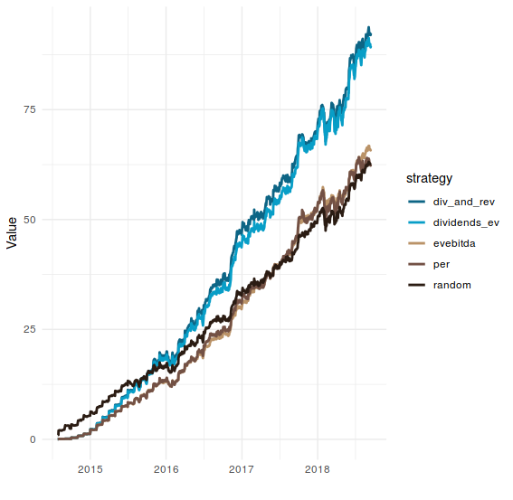
I know, I know. We are just taking a random subset of 100 companies instead of those juicy 1500. And the results obtained from here could be utterly different if we repeat the experiment for a different 100 companies.
In order to address that, we can simply iterate that process with new randomly selected universe of stocks every time and compute the difference in the yearly return of each simulation.
# Compute Internal Rate of Return
irr <- function(cash_flows, frequency = 30.5, error = 0.01){
	l <- length(cash_flows)
	cf_zero <- cash_flows[[1]]
	cf_final <- cash_flows[[l]]
	irr_bot <- -100
	irr_top <- 100
	npv <- 0
	while(abs(cf_final - npv) > error){
		npv <- 0
		irr_trial <- (irr_bot+irr_top)/2
		for(i in 1:(floor(l/frequency))){
			npv <- npv + cf_zero*((1 + irr_trial/100)^(i))
		}
		if(cf_final > npv) irr_bot <- irr_trial
		if(cf_final < npv) irr_top <- irr_trial
	}
	return(irr_trial/100)
}

# Compute relative Difference between the Return of the portfolio and the benchmark
alpha_ret <- function(portfolio, benchmark){
	r_port <- irr(portfolio)
	r_ben <- irr(benchmark)
	a <- (r_port - r_ben)/(r_ben)
	return(a)
}

# Compute beta with the benchmark
beta <- function(portfolio, benchmark){
	return(cov(portfolio,benchmark/sd(benchmark)^2))
}

# Compute Jensen's alpha with the benchmark
alpha <- function(portfolio, benchmark){
	r_port <- irr(portfolio)
	r_ben <- irr(benchmark)
	a <- (r_port - beta(portfolio, benchmark)*r_ben)
	return(a)
}

trials <- 50
n_stocks <- 100
specificity <- 25
alpha_result <- list()
diff_result <- list()

strategies_list <- c("random", "per", "evebitda", "dividends_ev", "div_and_rev")

for(t in 1:trials){

	stocks_universe <- getTickers("all") %>% sample(n_stocks) %>% intersect(list.files("data/"))
	files <- paste0("data/",stocks_universe)
	dt <- rbindlist(lapply(files, read_feather)) %>% filter(price >= 0.1) %>% data.table()
	investment <- simulate_multiple_strategies_fasto(data = dt, amount_to_invest = 1, strategies = strategies_list, specificity = specificity)

	for(s in strategies_list) {
		diff_result[[s]][[t]] <- alpha_ret(portfolio = investment[["results"]] %>% filter(strategy == s) %>% .$value,
																	 benchmark = investment[["results"]] %>% filter(strategy == "random") %>% .$value
		)
	}
}
And plot the result like that
diff_result %>%
	as_tibble() %>%
	melt() %>%
	ggplot(aes(x = as.factor(variable), y = value)) +
	geom_boxplot(aes(fill = variable), colour = "black", alpha = 0.35) +
	geom_point(aes(colour = variable), size = 2) +
	theme_minimal() +
	xlab("Strategy") +
	ylab("Returns Relative Difference")+
	scale_colour_hp(discrete = TRUE, house = "ravenclaw", direction = -1, name = "Strategy") +
	scale_fill_hp(discrete = TRUE, house = "ravenclaw", direction = -1, name = "Strategy")
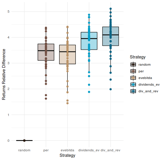
This plot shows the relative difference in the final yearly return between each strategy and the random. Obviously the random shows 0 difference with itself.
It is common to argue that simply higher returns does not equal to a better strategy, and that we should take into account the relative risk with respect with the benchmark. Since we are using the random selection as benchmark, we can use it like that and compute the Jensen’s Alpha for each strategy on every simulation (look the code above and note that this computation is hidden inside).
alpha_result %>%
	as_tibble() %>%
	melt() %>%
	ggplot(aes(x = as.factor(variable), y = value)) +
	geom_boxplot(aes(fill = variable), colour = "black", alpha = 0.35) +
	geom_point(aes(colour = variable), size = 2) +
	theme_minimal() +
	xlab("Strategy") +
	ylab("Alpha")+
	scale_colour_hp(discrete = TRUE, house = "ravenclaw", direction = -1, name = "Strategy") +
	scale_fill_hp(discrete = TRUE, house = "ravenclaw", direction = -1, name = "Strategy")
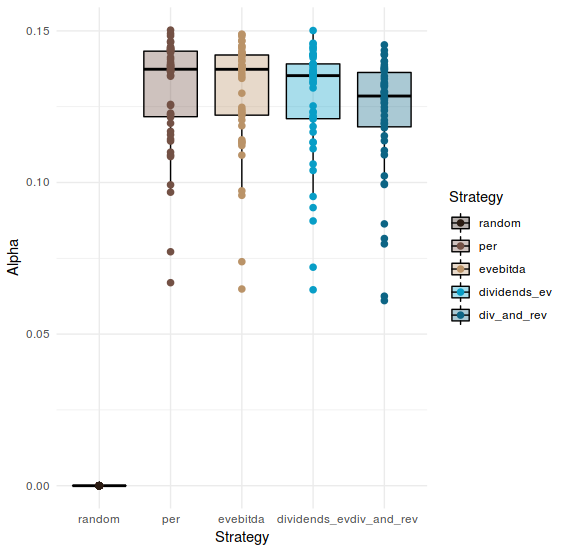
I don’t want to start arguing about whether we should look at the relative difference or the alpha in order to decide the preferred strategy, I think there are better discussion on that that the one I can provide in this essay. Nevertheless, seems quite obvious that the strategies that we have used contain some truth in them, they can outperform a random selection. So using them could better than blind random selection. I’m not sure if that is a big achievement, but it something; and can lead to further exploration of the utility of the metrics involved.
There are some biases that we should be aware of. Some of those could trigger further exploration of what I’ve done so far, trying to address them.
The most important one: Choosing the specificity parameter. The results can vary greatly if we change this parameter. Early exploration has shown me that if we set the specifity as 1, every strategy does not differ from the random, and we couldn’t say that they add value. I most certainly will expand the article in the future exploring this issue.
Universe of available stocks. We have chosen the lists of the standard and poors available today. This adds survivor bias, because we are only considering the companies that are in those lists nowadays, not back in 2014 or at every moment of the simulation. This is a problem because when we simulate being in 2014 with the information of 2014 we are not seeing the stocks that were in the lists of the SP back in 2014, but those that are present in the lists of 2018. We are using information of the future, and that is dangerous. I wouldn’t say is a big deal, because in 4 years these lists don’t change so much, but still.
Time. 4 years is simply not enough to extract reliable conclusions. Even though our datasets look huge, 4 years in financial history is just a small glimpse. This time range does not include periods of crisis, bursting of bubbles or any other major financial distress. Moreover, long-term saving strategies are thought to be applied during periods of more than 10 years; so even though we are claiming to simulate a real humble investor, the results we are providing can not applied to that situation. The reason why we only have 4 years is because I haven’t been able to retrieve older financial statements. I’ll work on that.